An Introduction to Linear Regression

In this post, we will be using a lot of Python. All of the code can be found here.

We'll be using data from R2D3, which contains real estate information about New York City and San Francisco real estate.

Regression

One of the most important fields within data science, regression is about describing data. Simply put, we will try to draw the best line possible through our data.

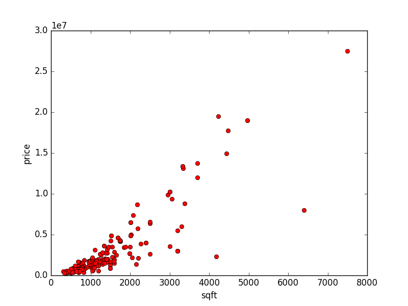
First, an example. Let's plot some New York City apartments' prices by square foot:

# c1_plot_ny.py
import csv

import matplotlib.pyplot as plt


def get_data():
    with open('ny_sf_data.csv', 'rb') as csvfile:
        reader = csv.DictReader(csvfile)
        rows = [r for r in reader]

        ny_data = [
            (int(p['sqft']), int(p['price']))
            for p in rows
            if p['in_sf'] == '0'
        ]
        return ny_data


def plot_data(data):
    sqft, price = zip(*data)
    plt.plot(sqft, price, 'ro')
    plt.xlabel('sqft')
    plt.ylabel('price')
    plt.show()


if __name__ == '__main__':
    data = get_data()
    plot_data(data)

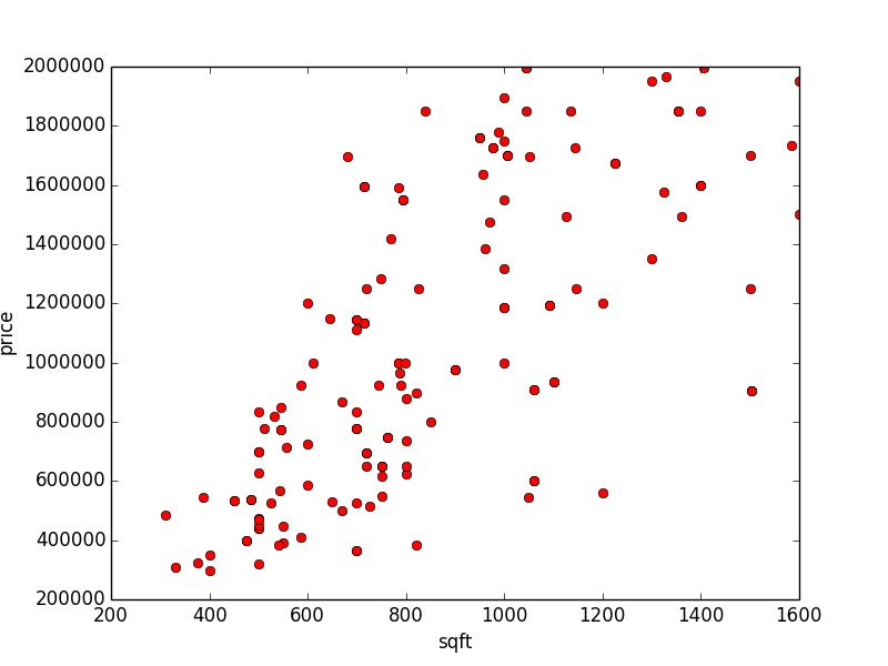
As you can see, there's a bit of bunching up in the lower left corner because we have a bunch of outliers. Let's say any apartment over $2M or 2000 square feet is an outlier (although, I think this is our dataset showing it's age...).

# c2_plot_ny_wo_outliers.py

from c1_plot_ny import get_data, plot_data


def get_data_wo_outliers():
    ny_data = get_data()
    ny_data_wo_outliers = [
        (s, p) for s, p in ny_data
        if s < 2000 and p < 2000000
    ]
    return ny_data_wo_outliers


if __name__ == '__main__':
    data = get_data_wo_outliers()
    plot_data(data)

Okay, so we can notice a couple things about this data:

There's a minimum number of square feet and price. No one has an apartment smaller than 250 square feet and no one has a price lower than 300K. This makes sense.
The data seems to go in a up-right direction, so we more or less draw a line naively if we tried.
As we go along the axes, the data spreads. There must be other variables at work.

Drawing our line

Let's try to draw the best straight line we can though the data. This is called linear regression. So our line is going to have the familiar-looking formula:

\begin{align} h_\theta(x) = \theta_0 + \theta_1 x \end{align}

Where $h_\theta(x)$ is our hypthesis $h$ of the price given a square foot of $x$ . Our goal is to find our $\theta$ s, which define the slope and y-intercept of our line.

So how do we define the best line? Through an cost function, which defines how off a line is! The line with the least cost is the best line.

Okay, so how do we choose an cost function? Well, there's a lot of different cost functions out there, but least squares error is perhaps the most common:

\begin{align} J(\theta) = {1 \over 2} \sum_{i=0}^n (h_\theta(x_i) - y)^2 \end{align}

Essentially, for each data point $(x_i, y_i)$ , we're simply taking the difference between $y_{i}$ and $h_\theta(x_i)$ and squaring it. Then we're summing them all together and halving it. Makes sense.

Gradient Descent

Okay, so now the hard part. We have data and a cost function, so now we need a process for reducing cost. To do this, we'll use gradient descent.

Gradient descent works by constantly updating any $\theta_j$ in the direction that will dimension $J(\theta)$ . Or:

\begin{align} \theta_j := \theta_j - \alpha {\delta \over \delta \theta_j} J(\theta) \end{align}

Where $\alpha$ is essentially "how far" down the slope you want to go at every step.

Thus, with a little bit of math, we can find the derivative of our $\theta_j$ with respect to $J(\theta)$ for an individual data point:

\begin{align} {\delta \over \delta \theta_j} J(\theta) &= {\delta \over \delta \theta_j} {1 \over 2} (h_\theta(x) - y)^2 \cr &= 2 \cdot {1 \over 2} \cdot (h_\theta(x) - y) \cdot {\delta \over \delta \theta_j} (h_\theta(x) - y) \cr &= (h_\theta(x) - y) \cdot {\delta \over \delta \theta_j} (h_\theta(x) - y) \end{align}

Now things begin to diverge for our $\theta$ s:

\begin{align} {\delta \over \delta \theta_0} J(\theta) &= (h_\theta(x) - y) \cdot {\delta \over \delta \theta_0} (\theta_0 + \theta_1 x - y) \cr &= (h_\theta(x) - y) \end{align}

\begin{align} {\delta \over \delta \theta_1} J(\theta) &= (h_\theta(x) - y) \cdot {\delta \over \delta \theta_1} (\theta_0 + \theta_1 x - y) \cr &= (h_\theta(x) - y) \cdot x \end{align}

So now we can apply our derivatives to the original algorithm...

\begin{align} \theta_0 := \theta_0 + \alpha (y - h_\theta(x)) \cr \theta_1 := \theta_1 + \alpha (y - h_\theta(x)) \cdot x \end{align}

However, this only applies to one data point. How do we apply this to multiple data points?

Batch Gradient Descent

The idea behind batch gradient descent is simple: go through your batch and get all the derivatives of ${\delta \over \delta \theta_0} J(\theta)$ . Then take the average:

\begin{align} \theta_0 := \theta_0 + \alpha \sum_{i=0}^m (y - h_\theta(x)) \cr \theta_1 := \theta_1 + \alpha \sum_{i=0}^m (y - h_\theta(x)) \cdot x \end{align}

This means that you only change your theta at the end of the batch:

# c3_batch_gradient_descent.py

import sys

import matplotlib.pyplot as plt

from c2_plot_ny_wo_outliers import get_data_wo_outliers


# Try playing with the learning rates!
THETA_0_LEARNING_RATE = 0.1
THETA_1_LEARNING_RATE = 0.1**6


def batch_gradient_descent(data, theta_0, theta_1):
    # End up with:
    # Iteration 316, error: 65662214541.7, thetas: 80241.5458922 1144.09527519
    N = len(data)
    error = 0
    theta_0_sum = 0
    theta_1_sum = 0
    for x, y in data:
        hypothesis = estimate_price(theta_0, theta_1, x)
        loss = y - hypothesis

        error += 0.5 * (loss) ** 2
        theta_0_sum += loss
        theta_1_sum += loss * x
    theta_0 += (THETA_0_LEARNING_RATE * theta_0_sum) / N
    theta_1 += (THETA_1_LEARNING_RATE * theta_1_sum) / N
    error /= N
    return error, theta_0, theta_1


def linear_regression(data, gradient_descent_func):
    theta_0 = 0
    theta_1 = data[0][1] / data[0][0]
    last_error = sys.maxint
    error = 1
    i = 0
    while (abs(error - last_error) / error) > (0.1 ** 7):
        last_error = error
        error, theta_0, theta_1 = gradient_descent_func(
            data, theta_0, theta_1
        )
        i += 1
        print 'Iteration {}, error: {}, thetas: {} {}'.format(i, error, theta_0, theta_1)

    return theta_0, theta_1


def estimate_price(theta_0, theta_1, x):
    return theta_0 + theta_1 * x


def plot_data_w_line(data, theta_0, theta_1):
    sqft, price = zip(*data)
    max_price, max_sqft = max(price), max(sqft)
    estimated_price = [estimate_price(theta_0, theta_1, x) for x in sqft]

    plt.plot(sqft, price, 'ro')
    plt.plot(sqft, estimated_price, 'b-')
    plt.axis([0, max_sqft, 0, max_price])
    plt.xlabel('sqft')
    plt.ylabel('price')
    plt.show()


if __name__ == '__main__':
    data = get_data_wo_outliers()
    theta_0, theta_1 = linear_regression(data, batch_gradient_descent)
    plot_data_w_line(data, theta_0, theta_1)

This results in:

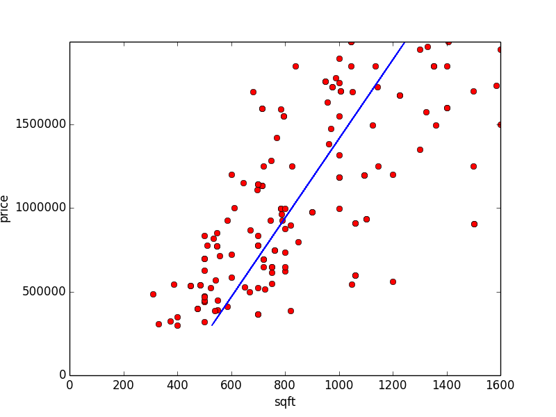
Pretty good! The code completes in 316 iterations, an error of 65662214541.7 and estimates $\theta_0$ to be 80241.5458922 and $\theta_1$ to be 1144.09527519.

Stochastic Gradient Descent

Another way to train our data is to apply our changes to each data point individually. This is stochastic gradient descent:

\begin{align} \theta_0 := \theta_0 + \alpha (y - h_\theta(x)) \cr \theta_1 := \theta_1 + \alpha (y - h_\theta(x)) \cdot x \end{align}

It has one big benefit: we don't have to go through the entire batch. This is hugely important for problems with large, large datasets. You'll see it used frequently in deep learning.

# c4_stochastic_gradient_descent.py

import random
import sys

import matplotlib.pyplot as plt

from c2_plot_ny_wo_outliers import get_data_wo_outliers
from c3_batch_gradient_descent import estimate_price, plot_data_w_line


# Try playing with the learning rates!
THETA_0_LEARNING_RATE = 0.1
THETA_1_LEARNING_RATE = 0.1**10


def stochastic_gradient_descent(data, theta_0, theta_1):
    # End up with:
    # Iteration 8075, error: 1.01475127545e+13, thetas: 103991.20381 1141.75031008
    error = 0
    for x, y in data:
        hypothesis = estimate_price(theta_0, theta_1, x)
        loss = y - hypothesis

        error += 0.5 * (loss)**2
        theta_0 = theta_0 + THETA_0_LEARNING_RATE * (y - hypothesis)
        theta_1 = theta_1 + THETA_1_LEARNING_RATE * (y - hypothesis) * x
    return error, theta_0, theta_1


def linear_regression(data, gradient_descent_func):
    theta_0 = 0
    theta_1 = data[0][1] / data[0][0]
    last_error = sys.maxint
    error = 1
    i = 0
    while (abs(error - last_error) / error) > (0.1**5):
        last_error = error
        random.shuffle(data)  # Try removing the randomness and see what happens :)
        error, theta_0, theta_1 = gradient_descent_func(
            data, theta_0, theta_1
        )
        i += 1
        print 'Iteration {}, error: {}, thetas: {} {}'.format(i, error, theta_0, theta_1)

    return theta_0, theta_1


if __name__ == '__main__':
    data = get_data_wo_outliers()
    theta_0, theta_1 = linear_regression(data, stochastic_gradient_descent)
    plot_data_w_line(data, theta_0, theta_1)

It's worth noting that this took longer than batch descent since our dataset is so small. Also, we had to loosen up the right answer since we oscillated around the error a lot more. We would oscillate a lot less if it weren't for the randomness!

There are in-betweens like mini-batch gradient descent, where you randomly turn your large dataset into small batches. This is hugely useful if you're doing regression across multiple machines!

Multivariate Linear Regression

Okay, now things start to get fun. At the moment, we're dealing with one input dimension (AKA "Simple" Linear Regression), which is great for getting started, but most datasets have more than one dimension. We can generalize our algorithm using linear algebra.

First, let's say that we have $n$ dimensions. Thus, when we treat every input $x$ as a vector, we get:

\overrightarrow{x}^{(i)} = \begin{bmatrix} x^{(i)}_1 \cr x^{(i)}_2 \cr \vdots \cr x^{(i)}_n \cr \end{bmatrix}

We can generalize our $m$ number of training vectors to be:

X = \begin{bmatrix} --- (\overrightarrow{x}^{(1)})^T --- \cr --- (\overrightarrow{x}^{(2)})^T --- \cr \vdots \cr --- (\overrightarrow{x}^{(m)})^T --- \cr \end{bmatrix}

And our answers, $y$ , can be a vector as well:

\overrightarrow{y} = \begin{bmatrix} y^{(1)} \cr y^{(2)} \cr \vdots \cr y^{(m)} \cr \end{bmatrix}

And our parameters as well:

\overrightarrow{\theta} = \begin{bmatrix} \theta_{1} \cr \theta_{2} \cr \vdots \cr \theta_{n} \cr \end{bmatrix}

We're losing our "error" parameter of $\theta$ . If you really want it, you can simply add a "1" column to each datapoint and that'll accomplish the same thing and allow us to simplify our math and code a bit.

So our hypothesis for an individual data point looks like:

\begin{align} h_\theta(\overrightarrow{x}^{(i)}) = (\overrightarrow{x}^{(i)})^T \cdot \overrightarrow{\theta} \end{align}

So going back to our cost function, which we can put in matrix form:

\begin{align} J(\theta) &= {1 \over 2} \sum_{i=0}^n (h_\theta(\overrightarrow{x}^{(i)}) - y^{(i)})^2 \cr &= {1 \over 2} (h_\theta(X) - \overrightarrow{y})^T(h_\theta(X) - \overrightarrow{y}) \cr &= {1 \over 2} (X \cdot \overrightarrow{\theta} - \overrightarrow{y})^T(X \cdot \overrightarrow{\theta} - \overrightarrow{y}) \end{align}

So if we wanted to find the derivative of $J(\theta)$ now (aka $\nabla_{\theta}J(\theta)$ ), we'd have to do some funky math. If you want to read how it can be derived, I recommend reading page 11 of Andrew Ng's lecture notes on Linear Regression.

Skipping to the answer, we get:

\begin{align} \nabla_{\theta}J(\theta) &= X^T(X \cdot \theta - \overrightarrow{y}) \end{align}

And thus, we can create steps for our $\overrightarrow{\theta}$ :

\begin{align} \overrightarrow{\theta} := \overrightarrow{\theta} + \alpha X^T(\overrightarrow{y} - (X \cdot \theta)) \end{align}

This kind of looks like our step for $\theta_1$ not too long ago!

\begin{align} \theta_1 := \theta_1 + \alpha (y - h_\theta(x)) x \end{align}

Programming this in numpy

# c5_stochastic_gradient_descent.py

import random
import sys

import matplotlib.pyplot as plt
import numpy as np

from c2_plot_ny_wo_outliers import get_data_wo_outliers
from c3_batch_gradient_descent import estimate_price, plot_data_w_line


LEARNING_RATE = 0.1**6


def batch_gradient_descent(x, y, theta):
    # End up with:
    # Iteration 8, error: 9.643796593e+12, theta: [    2.35848572  1227.94035952]
    x_trans = x.transpose()
    M = len(x)
    hypothesis = np.sum(x * theta, axis=1)
    loss = hypothesis - y
    theta -= LEARNING_RATE * (np.sum(x_trans * loss, axis=1)) / M
    error = np.sum(0.5 * loss.transpose() * loss)
    return error, theta


def linear_regression(x, y, gradient_descent_func):
    theta = np.ones(np.shape(x[0]))
    last_error = sys.maxint
    error = 1
    i = 0
    while (abs(error - last_error) / error) > (0.1 ** 7):
        last_error = error
        error, theta = gradient_descent_func(
            x, y, theta
        )
        i += 1
        print 'Iteration {}, error: {}, theta: {}'.format(i, error, theta)

    return theta


def data_in_np(data):
    sqft, price = zip(*data)
    # Adding a 1 to replicate our \theta_0
    sqft = np.array([np.array([1, s]) for s in sqft])
    price = np.array(price)
    return sqft, price


if __name__ == '__main__':
    data = get_data_wo_outliers()
    sqft, price = data_in_np(data)
    theta = linear_regression(sqft, price, batch_gradient_descent)
    theta_0, theta_1 = theta
    plot_data_w_line(data, theta_0, theta_1)

We get a slightly different answer here than in our old batch gradient descent code because our y-intercept has a different learning rate. If we gave it enough repititions, it would eventually get near the same area.

Of course, there are plenty of high level ML libraries to explore that do this stuff for you! However, it's fun to understand what's happening under the hood.

Things to worry about

Multivariable linear regression with gradient descent can have a lot of complications. For example, local minima:

Example of a local minima. Source: Creative Commons

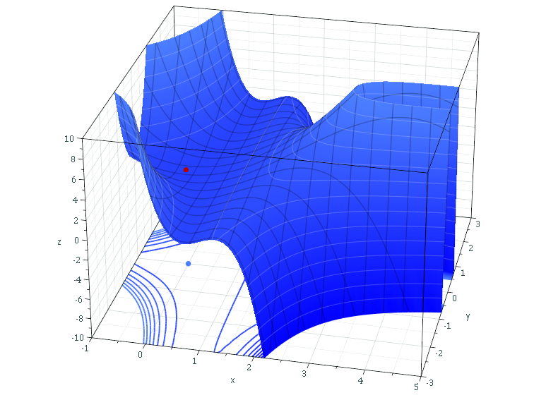
As you can see, gradient descent might accidentally think the minimum is in the saddle there. There's a ton of interesting papers about this. Training multiple times with different starting parameters is one way around this.

Overfitting is also an issue:

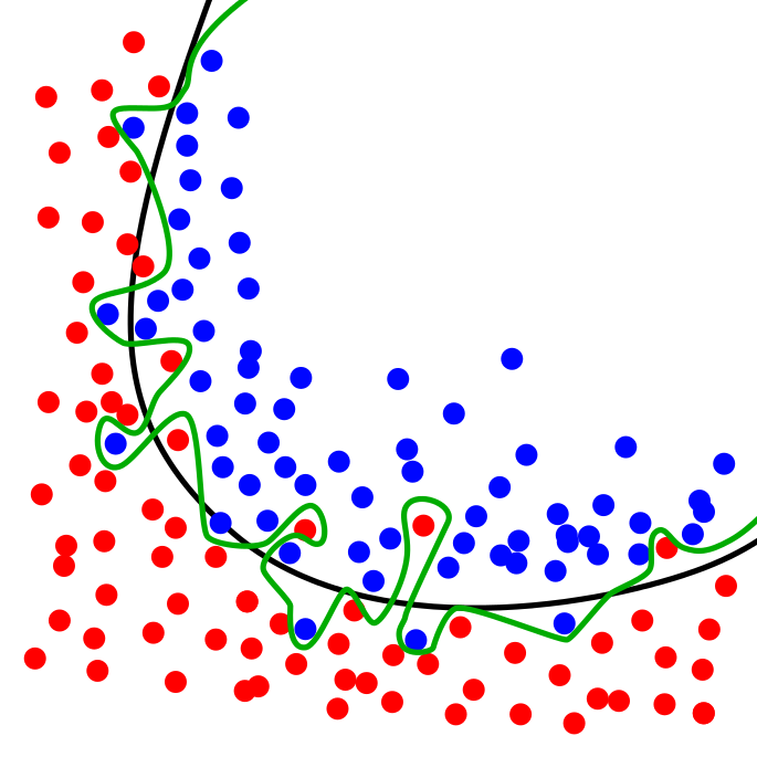
You can avoid this by splitting your data into a large "training" set and a large "testing" set. That's standard procedure in most data science problems.

One last method: using the derivative

As many of you know, if you set the derivative of a curve to 0, it'll either be a local maxima or a local minima. Since our error function does not have an upper limit, we know that the point where the derivative is 0 is a local minima.

So we can make our derivative $\nabla_{\theta}J(\theta)$ zero:

\begin{align} \nabla_{\theta}J(\theta) &= X^T(X\theta - \overrightarrow{y}) \cr 0 &= X^T(X\theta - \overrightarrow{y}) \cr X^TX\theta &= X^T\overrightarrow{y} \cr \theta &= (X^TX)^{-1}X^T\overrightarrow{y} \end{align}

And we can throw it in our code:

# c6_derivative_method.py

import random
import sys

import matplotlib.pyplot as plt
import numpy as np

from c2_plot_ny_wo_outliers import get_data_wo_outliers
from c3_batch_gradient_descent import estimate_price, plot_data_w_line


LEARNING_RATE = 0.1**6


def linear_regression(x, y):
    # End up with 82528.3036581 1141.67386409 :)
    x_trans = x.transpose()
    return np.dot(np.linalg.inv(np.dot(x_trans, x)), np.dot(x_trans, y))


def data_in_np(data):
    sqft, price = zip(*data)
    sqft = np.array([np.array([1, s]) for s in sqft])
    price = np.array(price)
    return sqft, price


if __name__ == '__main__':
    data = get_data_wo_outliers()
    sqft, price = data_in_np(data)
    theta = linear_regression(sqft, price)
    theta_0, theta_1 = theta
    print theta_0, theta_1
    plot_data_w_line(data, theta_0, theta_1)

And it totally works! You may ask "but why did we learn all about the gradient descent stuff then"? Well, you'll need it for things that aren't as straight forward as linear regression like deep neural networks.

To learn more:

Andrew Ng's notes on Linear Regression.

ML @ Berkeley's Machine Learning Crash Course.